Basic Tutorial

There are 3 steps to estimate satellite brightness:

1. Find BRDFs for the surfaces of a satellite and Earth’s surface

2. Create a brightness model based on BRDFs, normal vectors, and surface areas

3. Calculate brightness

This tutorial will walk you through each of these steps and give you some basic background knowledge about the most important concepts underlying the Lumos brightness calculations. For a more formal and detailed information, see our paper Satellite Optical Brightness (2023)

For the purposes of this tutorial, instead of a complex satellite, we’ll use a 5 square meter aluminum plate. This is a very simple test case.

Installation

First, create a new directory:

$ mkdir lumos_tutorial
$ cd lumos_tutorial

Create a Python virtual environment:

$ python -m venv venv
$ venv/Scripts/activate.bat

Install Lumos using pip:

(.venv) $ pip install lumos-sat

Bidirectional Reflectance Distribution Function (BRDF)

The BRDF describes how light is scattered by a surface. Shiny or glossy materials such as polished aluminum have a specular BRDF. Surfaces like this mostly scatter light in the direction of perfect reflection. Diffuse materials such as a white piece of paper have a nearly Lambertian BRDF, meaning light is scattered equally in allows directions.

We need to know the BRDF for each surface of our satellite. This is one of the most important parts of generating an accurate brightness model. The best way to go about this is to fit BRDF data that has been measured in the lab to an empirical BRDF model. Fitting data to an empirical model is useful because it can help get rid of measurement artifacts and is safer than extrapolating a small number of BRDF measurements over a huge variety of angles.

Let’s find a BRDF model for our aluminum plate. Start by downloading this CSV file Aluminum BRDF Data and placing this file in your working directory. This BRDF data is from a catalog provided in the paper “A Data-Driven Reflectance Model (Matusik et. al 2006)”

Note

Lumos uses a very specific BRDF file format. The first column is the ingoing zenith angle \(\phi_{in}\). The second column is the ingoing azimuth angle \(\theta_{in}\). The third and fourth columns are the outgoing angles \(\phi_{out}\), \(\theta_{out}\). The fifth column is the BRDF. The delimiter should be five spaces. Comments can be written using “#”. See the aluminum BRDF file you just downloaded as an example.

Since we are working with aluminum, we’ll fit our experimental BRDF data to an ABG model. The ABG model is good for representing specular BRDFs. The model consists of three parameters we need to fit: A, B, and g. You can read more about the ABG model here: Scatter Models for Stray Light Analysis We use lumos.brdf.tools.fit() to find these three model parameters:

fit_aluminum_brdf.py

import numpy as np
import lumos.brdf.tools
import matplotlib.pyplot as plt
import lumos.plot
from lumos.brdf.library import ABG

A, B, g = lumos.brdf.tools.fit(
    "examples/aluminum_brdf.csv",
    ABG,
    bounds = (0, 1e4),
    p0 = (1, 1, 1))

print(f"{A = :0.3e}")
print(f"{B = :0.3e}")
print(f"{g = :0.3f}")

A = 3.362e-03
B = 4.309e-06
g = 2.068

Next, we use Lumos to plot both our measured data points and our fitted model. This is an important step to ensure we have a good fit.

fit_aluminum_brdf.py

fig, ax = plt.subplots()

phi_i, theta_i, phi_o, theta_o, brdf = lumos.brdf.tools.read_brdf("examples/aluminum_brdf.csv")
ax.semilogy(phi_o, brdf, 'k.', alpha = 0.5, zorder = 2)
lumos.plot.BRDF_1D(ax, ABG(A, B, g), incident_angles = np.unique(phi_i))

plt.xticks(fontsize = 14)
plt.yticks(fontsize = 14)
plt.xlabel("Outgoing Zenith Angle", fontsize = 16)
plt.ylabel(r"BRDF $(sr^{-1})$", fontsize = 16)
plt.title("Aluminum BRDF", fontsize = 20)
plt.legend(fontsize = 14)
plt.show()

Our fitted BRDF model looks good! Next, we can make a satellite model.

Note

For more complex BRDFs, you will most likely want to use a Binomial model. Be careful when fitting binomial models, as these fits can easily “go wild” outside of measurements.

Making a Satellite Model

For our brightness modeling, we treat a satellite as a collection of surfaces. Each surface is defined by a normal vector, BRDF, and surface area.

The normal vector of a surface must be given in the “satellite-centered frame”. In this reference frame, \(\hat{z}\) points to zenith. \(\hat{y}\) is in the plane defined by the center of earth, the satellite, and the sun. \(\hat{x}\) is defined by the right-hand-rule. We also define angle \(\alpha\), the angle of the satellite past the terminator (night-day boundary). All of this geometry is shown below:

Note

For example, the vector that points straight down (to geodetic nadir) from a satellite, usually corresponding to the underside of the satellite chassis would be: \(\hat{n} = -\hat{z} = (0, 0, -1)\).

The vector that points from the satellite directly to the sun is given as: \(\hat{n} = \hat{y} \cos \alpha - \hat{z} \sin \alpha = (0, \cos \alpha, -\sin \alpha)\).

Let’s make a new brightness model, consisting of just our aluminum plate, pointing towards the ground. We start by making a new file, “simple_sat.py”, where we define the surfaces of our model.

simple_sat.py

from lumos.geometry import Surface
from lumos.brdf.library import ABG
import numpy as np

area = 5.0     # meters^2
normal = np.array([0, 0, -1])
brdf = ABG(A = 3.362e-03, B = 4.309e-06, g = 2.068)

aluminum_plate = Surface(area, normal, brdf)

SURFACES = [aluminum_plate]

Next, we can use this model to generate some brightness predictions.

The Satellite-Centered Frame

Lumos provides a very simple interface to generate brightness predictions in the satellite frame.

aluminum_satellite_frame.py

import simple_sat
import lumos.plot
import lumos.brdf.library
import numpy as np

sat_height = 550 * 1000 # Geodetic height of satellite (meters)

angles_past_terminator = [5, 10, 15, 20]

lumos.plot.brightness_summary_satellite_frame(
    simple_sat.SURFACES,
    angles_past_terminator,
    sat_height,
    levels = (3, 10)
    )

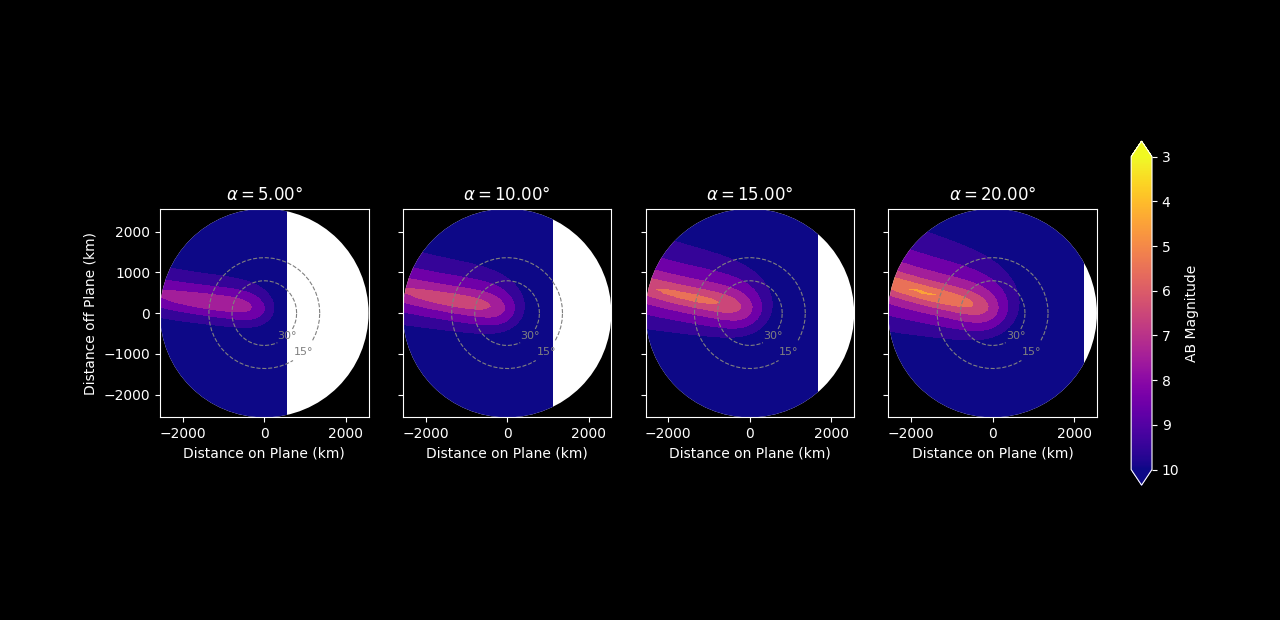
Let’s unpack this image a bit. We are in the satellite’s frame of reference, looking down on the Earth’s surface. The outer circle shows the horizon seen by the satellite, everything outside of this circle is space. Observers on this circle would see the satellite exactly at the horizon. The dashed-grey concentric circles mark observers on the ground, who, when looking at the satellite, see it at altitudes of 15 and 30 degrees respectively. The white semi-circle to the left of each frame shows the portion of the Earth which is still illuminated by the sun. The vertical boundary between night and day is the terminator. The bright streak to the right hand side of the images shows light scattered by our aluminum plate.

As the angle past terminator increases, more light is scattered for two reasons. First, the aluminum plate’s normal vector is oriented more directly towards the sun. Second, the scattered light seen by observers on the ground is being reflected more and more specularly. Here’s an interactive graph showing how this works:

While this reference frame may seem overly complicated, it is actually very useful when thinking about satellite designs. As an example, let’s try changing the normal vector of our aluminum surface. First, we rotate the aluminum in the x-direction:

aluminum_satellite_frame.py

# Angle of rotation of the surface
angle = np.deg2rad(20)

# Rotate the surface in the x direction
simple_sat.SURFACES[0].normal = np.array([np.sin(angle), 0, -np.cos(angle)])

lumos.plot.brightness_summary_satellite_frame(
    simple_sat.SURFACES,
    angles_past_terminator,
    sat_height,
    levels = (3, 10)
    )

We can see how our surface now scatters light into the x-hat direction.

Let’s rotate the aluminum 45 degrees in the y-direction. Now our specular peak is below the satellite!

aluminum_satellite_frame.py

# Angle of rotation of the surface
angle = np.deg2rad(45)

# Rotate the surface in the y direction
simple_sat.SURFACES[0].normal = np.array([0, np.sin(angle), -np.cos(angle)])

lumos.plot.brightness_summary_satellite_frame(
    simple_sat.SURFACES,
    angles_past_terminator,
    sat_height,
    levels = (3, 10)
    )

The following interactive graph shows how light is specularly scattered onto the ground by our rotated aluminum plate:

What if, instead of just plotting a brightness summary, we want to get the actual intensity values calculated by Lumos? We simply call the calculation directly. Here’s an example which calculates the location of the observer that sees the brightest reflection from the aluminum and the peak intensity of that reflection.

aluminum_satellite_frame.py

import lumos.geometry
observers = lumos.geometry.GroundObservers(
                sat_height,
                np.deg2rad(20),
                density = 200
            )

observers.calculate_intensity(simple_sat.SURFACES)

idx = np.argmax( observers.intensities )
dist_off_plane = observers.dists_off_plane.flatten()[idx]
dist_on_plane = observers.dists_on_plane.flatten()[idx]

print( f"Peak Intensity: {observers.intensities.max() * 1e9:0.0f} nW / m^2")
print( f"Distance off Plane: {dist_off_plane / 1000 :0.0f} km")
print( f"Distance on Plane: {dist_on_plane / 1000 :0.0f} km")

Peak Intensity: 130 nW / m^2
Distance off Plane: -13 km
Distance on Plane: 207 km

This matches the contour plot shown above. See the API reference for more information about what is included in a lumos.geometry.GroundObservers object.

The satellite-centered frame is great for satellite operators, since this frame shows how design decisions affect brightness in the frame of a satellite. On the other hand, astronomers would like to know how satellite brightness will impact the night sky. For this, we use a different reference frame.

The Observer Frame

In the observer frame, the position of a satellite in the sky and the position of the sun in the sky are both specified by their altitude and azimuth. Altitude is the angle in degrees of an object from the horizon. Azimuth is the angle of the object from due north. Internally, Lumos converts these sky positions to coordinates in the brightness frame, then calculates brightness.

Let’s see an example using our nadir-facing aluminum plate:

aluminum_observer_frame.py

import simple_sat
import lumos.plot

lumos.plot.brightness_summary_observer_frame(
    simple_sat.SURFACES,
    sat_height = 550 * 1000,
    sun_altitudes = [-3, -9, -15, -21, -27],
    sun_azimuths = [90, 90, 90, 90, 90],
    levels = (3, 10)
)

Warning

You must always specify exactly 5 sun altitudes and 5 sun azimuths for lumos.plot.brightness_summary_observer_frame() to work.

So what does this image show? Each circle shows a view of the entire night sky. The contour color is filled according to the brightness a satellite would appear if it was in that point in the sky. The center corresponds to a satellite straight overhead. North, West, South, and East are marked on the edge of the circle (which is the horizon). Altitude is shown in increments of 10 degrees. As an example, we see that when the sun is at -27 degrees, the brightest satellites would be in the eastern sky, about 25 degrees above the horizon. This light is forward scattered by our nadir aluminum plate. In most of the western sky and directly overhead, satellites are shadowed by Earth.

To get numerical intensity values we can call the Lumos calculator directly:

aluminum_observer_frame.py

import lumos.calculator
import numpy as np

sat_height = 550 * 1000 # 550 kilometer geodetic height


sat_altitudes, sat_azimuths = \
    np.meshgrid(
    np.linspace(0, 90, 90), 
    np.linspace(0, 360, 180))

intensities = lumos.calculator.get_intensity_observer_frame(
        simple_sat.SURFACES, sat_height, sat_altitudes, sat_azimuths,
        sun_altitude = -27, sun_azimuth = 90,
        include_earthshine = False
    )
    
# Convert intensity to AB Magnitude
ab_magnitudes = lumos.conversions.intensity_to_ab_mag(intensities)

peak_ab_mag = ab_magnitudes.min()
idx = np.argmin(ab_magnitudes)
peak_alt = sat_altitudes.flatten()[idx]
peak_az = sat_azimuths.flatten()[idx]

print( f"Brightest: {peak_ab_mag:0.1f} AB Magnitude")
print( f"Altitude: {peak_alt:0.0f}°")
print( f"Azimuth: {peak_az:0.0f}°")

Brightest: 4.6 AB Magnitude
Altitude: 23°
Azimuth: 91°

Note

To find the altitude and azimuth of the sun at a specific time and location, you can use lumos.calculator.get_sun_alt_az(). You must pass in an astropy.time.Time object and a astropy.location.EarthLocation object.

Conclusion

That wraps up everything you need to know for the most basic usage of Lumos. Head over to Advanced Topics for more helpful tips.